
The Mathematical Architecture of Technological Revolution
A Mathematical Analysis of Perezian Cycle Dynamics
Perez’s framework is translated into the following equations for those who grasp new concepts more easily through mathematical equations. No worries, every element of the equations is explained so that even a layman can readily understand and follow along with the math. Using this approach demonstrates the Models’ Math Consistency
The mathematical framework presented represents a groundbreaking attempt by AI systems to quantify the complex dynamics that govern technological revolutions. Utilizing Carlota Perez’s modeling of techno-economic paradigm shifts, these equations provide a mathematical foundation for understanding how technological cycles unfold across decades and centuries.
One of the crucial factors that must be understood is that history is always unique each time, but the forces driving innovation remain the same. Those forces are structural. This is why Carlota’s framework is so valuable. It allows for the flexibility of history and captures the underlying structure.
The forces are constant while the manifestations are always unique. It is like gravity: the force is always the same, but how objects fall depends on their shape, the medium they are falling through, and countless other variables.
The underlying forces driving technological cycles are always:
Innovation clustering and network effects
Capital seeking profitable opportunities with the shortest return times
Social systems struggling to adapt to new realities
Institutional rigidity creates tensions that eventually break
These forces are structural constants – they operate the same way whether we are talking about steam railways in the 1840s, electricity in the 1880s, or the Microprocessor in the late 1980s.
But the historical content – the specific technologies, the particular social conflicts, the unique cultural responses, the individual political crises – that is all completely different each time because humans are creative, adaptive beings operating in other contexts.
This is why Perez’s model is mathematically elegant and historically realistic. It captures:
The invariant mathematical structure (the four phases, the energy dynamics, the transition patterns)
The variable historical content (the specific ways each society responds to technological transformation)
Most theories fail because they are either too rigid (trying to predict specific outcomes) or too flexible (saying “anything can happen”). Perez struck a balance, constructing a predictable model that identifies the deep structural forces while allowing for infinite historical creativity in how those forces play out.
It is like having a map that shows you the terrain (the forces) while letting you choose your path through it (the history).
The four equations we will explore represent four distinct phases of technological revolution: the Gestation (Core Formation), Installation, Turning Point, and Deployment Periods. Each phase has its mathematical signature, rhythm, and pattern. Together, they form what we might call the “mathematical choreography” of technological change—a dance that has repeated throughout history and will continue to shape our future.
This mathematical treatment transforms Perez’s qualitative observations into quantifiable relationships, offering unprecedented precision in modeling technological change. We use examples from the first technology cycle – the Industrial Revolution – because the complexity was lowest.
Mathematical Framework: The Four Periods
Gestation – The Core Formation Period
The Genesis of Innovation
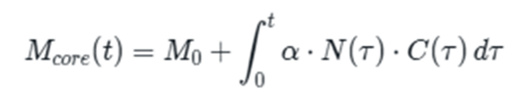
The Core Formation Period represents the foundational phase where scattered innovations begin to coalesce into a coherent technological system. The equation for Core Formation captures the accumulation of technological capability over time through an integral formulation that reflects the cumulative nature of innovation.
The mathematical structure incorporates several crucial parameters. The initial innovation base represents pre-existing technological knowledge, reflecting that technological revolutions build upon previous achievements. The innovation rate function exhibits characteristic patterns starting modestly, perhaps two or three major innovations annually early, but accelerating to eight or ten annually by the latter stages.
The period revealed distinct phases: scattered innovation with limited interconnection early, increasing rates with growing connections in the middle of the period, followed by high rates with strong clustering effects, setting the stage for the coming Installation dynamics.
Do not let the mathematical symbols intimidate you. This equation is telling a very human story about how innovations come together to create something revolutionary. Let us break down the variables one at a time.
Reviewing the Gestation periods variables
Mcore(t) represents the “technological mass” that accumulates over time. Think of this as the combined weight of all the innovations, discoveries, and improvements that are clustering together. In the case of the steam and railway revolution, this would encompass everything from enhancements in iron smelting techniques to advancements in precision tooling, from a deeper understanding of steam pressure to innovations in mechanical engineering.

M0 is where we start—the initial foundation of existing knowledge and technology. For the steam revolution, this was the basic understanding of steam power that existed, along with existing metallurgy techniques and mechanical knowledge. This is the technological “seed” from which the revolution will grow.

The integral sign (∫) might look intimidating, but it’s simply mathematical shorthand for “adding up over time.” It’s like saying, “Take all the innovations that happen between now and some future time, and add them all together.” The process of technological accumulation is continuous—it doesn’t happen in sudden jumps but rather through countless minor improvements and discoveries that build upon each other day by day, year by year.

The Greek letter α (alpha) represents the efficiency of innovation integration. This measures the effectiveness with which innovations are integrated into the expanding technological cluster. Some societies and periods are better at this than others. Britain in the early 1800s was particularly good at it—they had a culture that valued practical experimentation, a growing community of skilled artisans and engineers, and economic conditions that rewarded innovation. Other societies might generate individual innovations but struggle to integrate them effectively into a coherent technological system. France was a good example of the many valuable innovations invented after the Industrial Revolution began. But Britain deployed the innovations instead.

N(τ) represents the rate at which innovations are being created at any given time. Some periods are more fertile for innovation than others. During the late 18th and early 19th centuries, for instance, there was a surge of mechanical innovation in Britain. The number of patents being granted was increasing rapidly, and workshops across the country were buzzing with experimentation. This rate of innovation wasn’t constant—it accelerated as more people became involved and as existing innovations created opportunities for new ones.

C(τ) is perhaps the most crucial element: the clustering coefficient. The second symbol is the Greek symbol called Tau. It represents time. The coefficient measures how well innovations connect with and reinforce each other. Individual innovations, when isolated, have a limited impact. But when innovations begin to cluster—when improvements in metallurgy enable better steam engines, which in turn allow better transportation, which opens new markets, which creates demand for more innovations—the effect becomes exponential. The clustering coefficient captures this network effect, measuring how densely interconnected the innovations are becoming.

In the Core Formation equation, dτ represents each tiny slice of time—perhaps a day, a week, or a month—during which innovations are accumulating. Think of it this way: every single day during these 41 years, something was happening in British workshops, laboratories, and foundries. On one particular day in 1764, James Hargreaves might have made a crucial adjustment to his spinning jenny. On another day in 1769, James Watt could have achieved his breakthrough with the separate condenser.
The dτ captures each of these individual moments and ensures they all get counted in the total accumulation. Without dτ, we would only have rates—”innovations per year”—but we need the actual total mass of innovation that builds up over time. The dτ transforms those daily rates of discovery into the cumulative technological mass that eventually reached critical density. The dτ is what allows the mathematical integration to add up all those individual moments of innovation into the total technological mass that triggered the oncoming Installation Period.
Expanded Equation Explanation
Let us trace the Core Formation period of the steam and railway revolution from 1780 to 1829. At the beginning of this period, M0 was relatively small—some basic steam engines existed, primarily for pumping water out of mines. The iron industry was developing, but still primitive. Transportation was still largely dependent on horses, rivers, and wind.
However, the mathematical process described by our equation then began to unfold. The rate of innovation (N) began to accelerate. James Watt’s improvements to the steam engine in the 1770s and 1780s sparked a wave of further innovations. Each improvement created opportunities for others. Better steam engines required better metallurgy, which led to innovations in iron and steel production. More efficient steam engines opened new applications beyond mining—they could power textile mills, enabling the growth of industrial manufacturing.
The clustering coefficient (C) began to increase dramatically. Innovations in steam power related to innovations in metallurgy. Both are closely tied to innovations in precision tooling and mechanical engineering. These clusters began to suggest entirely new possibilities—if steam could power mills, why not vehicles? If steam vehicles were possible, why not lay down tracks to make them more efficient?
The integration efficiency (α) was high because Britain had developed an ecosystem that could absorb and build upon innovations. Skilled craftsmen could implement new techniques, entrepreneurs could identify commercial opportunities, and capital markets could fund development. The scientific societies shared knowledge, the patent system protected inventors, and economic conditions created strong incentives for practical innovation.
As this process continued year after year, the technological mass (Mcore) grew denser and more organized. By the 1820s, all the essential components of a railway system existed—steam engines powerful enough to pull carriages, iron rails strong sufficient to support them, engineering techniques capable of building bridges and tunnels, and financial instruments capable of funding large projects. The “mass” of accumulated innovations had reached a critical threshold.
This is where our equation becomes particularly illuminating. The integral nature of the accumulation process means that technological revolutions do not emerge suddenly—they build gradually over decades. But there comes a point where the accumulated mass becomes so dense, so interconnected, that it reaches a kind of critical mass. At this point, the slow accumulation of the Core Formation of the Gestation period gives way to the explosive energy release of the Installation Period.
The mathematics here mirrors what physicists call a phase transition, like water suddenly turning to steam when it reaches a critical temperature. For decades, innovations have accumulated gradually. The process seems slow, even dull. But then, suddenly, the accumulated mass converts to energy, and a technological revolution is born.
Understanding this mathematical process helps us recognize that technological revolutions are not accidents or mysteries—they are the inevitable result of innovation accumulation reaching a critical threshold. The steam revolution of the 1830s was not a sudden surprise, but the predictable outcome of decades of mathematical accumulation, as described by our Core Formation equation.
Installation Period
Explosive Growth and Creative Destruction
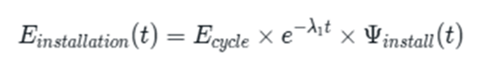
The Installation Period marks the transition from gradual accumulation to explosive deployment of new technologies. The equation for Installation captures this through exponential dynamics combined with oscillating disruption functions, modeling the boom-bust cycles characteristic of revolutionary technological change.
The mathematical structure begins with the total cycle energy term representing accumulated innovation potential from Core Formation seeking expression in the real economy. The exponential decay component reflects paradoxical Installation dynamics: while explosive growth occurs, the easiest implementation opportunities are rapidly depleted, requiring increasingly sophisticated approaches and facing greater resistance from established systems.
The oscillating disruption function models boom-bust cycles reflecting conflict between emerging technological possibilities and existing economic, social, and institutional structures. Each boom represents investment waves in new technologies, while busts represent painful adjustments as unrealistic expectations meet practical constraints.
Historical validation comes from the textile manufacturing’s explosive growth during the 1770s. Arkwright’s water frame technology spread from one mill in 1771 to over 200 by 1781—exponential growth with a 2.5-year doubling time. However, the 1781-1783 crisis brought price collapses and mill bankruptcies, followed by repeated boom-bust patterns in 1772-1773, 1783-1784, and 1792-1793.
Steam engine deployment showed similar patterns. Boulton and Watt engines increased from 5 installations in 1775 to over 500 by 1800, exhibiting clear boom-bust cycles corresponding to economic crises and recoveries. London financial markets experienced major bubbles and crashes corresponding to technological deployment cycles.
The social disruption was equally dramatic. Traditional artisans found their skills obsolete as mechanized production expanded. Geographic development concentrated in specific regions—Lancashire for textiles, the Black Country for metallurgy, Clydeside for chemicals—creating industrial districts with distinct characteristics but also vulnerabilities to downturns.
Creative destruction was particularly pronounced in the textiles industry, where mechanized production systematically displaced traditional cottage industries. Factory systems emerged, requiring new management, labor discipline, and accounting methods—organizational innovations as important as technological ones.
This equation describes a phenomenon we’ve all witnessed in various forms: the boom-and-bust cycle that characterizes the introduction of revolutionary technologies. Let us decode what each part means and how it played out during the steam and railway revolution of 1829-1848.
Reviewing the Installation periods variables
Einstallation(t) represents the total energy being released by the technological revolution at any given time during the Installation Period. This isn’t just economic energy—it’s social, political, and cultural energy as well. Think of it as the combined force of all the changes that the new technology is driving through society. During the railway installation period, this energy manifested as frenzied construction activity, massive financial speculation, social upheaval, political transformation, and cultural revolution.

Ecycle is the total energy that was stored up during the Core Formation period—essentially, all that accumulated technological mass converting into kinetic energy according to something like Einstein’s famous equation E=mc². This represents the total transformative potential of the new technology. For the steam and railway revolution, this was enormous. Railways didn’t just change transportation; they revolutionized manufacturing, agriculture, finance, urban development, social relations, and even people’s conception of time and space.

The term e^(-λ₁t) is where the mathematics becomes particularly revealing. This is an exponential decay function, and it captures one of the most critical and counterintuitive aspects of the Installation Period. While the energy release is initially explosive, it follows a pattern of exponential decay. The “e” here is Euler’s number (approximately 2.718), which appears throughout nature in processes involving growth and decay. The negative sign indicates that this is a decay process, and λ₁ (lambda) is the decay constant—a measure of how quickly the initial explosive energy burns through.
This might seem contradictory at first. How can a decay function describe a period of explosive growth? The answer lies in understanding what’s happening during the Installation Periods. The initial energy release is indeed massive, but it’s not sustainable at that level. The energy burns chaotically, often wastefully, and gradually dissipates. Think of it like a bonfire—the initial flames are highest, but without constantly adding fuel, they gradually die down.
During the railway installation period, this pattern is visible. The initial explosion of railway construction in the 1830s and early 1840s was extraordinary. In Britain, railway mileage expanded from virtually nothing to over 6,000 miles in less than two decades. But this growth was chaotic and inefficient. Multiple competing companies built redundant lines. Speculation ran wild. The famous “Railway Mania” of the 1840s saw investors pour money into railway schemes with reckless abandon, many of which were financially unsound or technically unfeasible.
The exponential decay aspect of the equation captures how this initial explosive energy gradually burned through. The easy opportunities were exploited first. The most obvious routes were built. The most enthusiastic investors were drawn in. However, as time passed, the remaining opportunities became increasingly challenging and expensive. The easy money was made, and the hard work of building a sustainable railway system remained.
This is where Ψinstall(t) (the Greek letter psi) becomes crucial. This represents the “oscillating disruption function”—the boom-and-bust cycles that characterize Installation Periods. Unlike the smooth exponential decay of the main energy release, this function captures the chaotic, oscillating nature of how energy is consumed by society.
Installation Periods are not smooth processes. They’re characterized by wild swings between euphoria and despair, between over-investment and panic withdrawal, between revolutionary optimism and reactionary backlash. The railway installation period exemplified this pattern. Periods of frenzied construction and speculation alternated with financial crashes and periods of skepticism. The Railway Mania of the 1840s was followed by the railway panic of 1847, which contributed to the broader economic crisis of that year.
These oscillations aren’t random—they follow mathematical patterns. The disruption function captures the feedback loops that drive boom-and-bust cycles. Initial success attracts more investment, which drives further construction, which in turn appears to validate the success, attracting even more investment. This positive feedback loop drives the “boom” phase. However, the system eventually becomes overextended. Reality fails to match expectations. A triggering event causes sentiment to shift, and the positive feedback loop becomes negative. Panic selling drives down prices, which justifies more panic selling, which drives prices down further.
The combination of exponential decay and oscillating disruption creates a characteristic pattern: a series of increasingly smaller boom-and-bust cycles. Each cycle burns through some of the revolutionary energy, but each successive cycle is smaller than the last. This continues until the energy is largely exhausted and the system reaches a crisis point—what Perez calls the Turning Point.
The mathematical beauty of this equation is that it explains why Installation Periods are simultaneously periods of tremendous progress and tremendous instability. The same energy that drives revolutionary change also drives speculation, overinvestment, and eventual crisis. This isn’t a bug in the system—it’s a feature. The chaotic energy of the Installation Period is necessary to break down old structures and create space for new ones.
The equation also helps us understand why Installation Periods inevitably end in crisis. No matter how revolutionary the technology, the chaotic energy of the Installation Period cannot be sustained indefinitely. The exponential decay ensures that the energy will eventually burn through, and the oscillating disruption ensures that the final oscillation will be a major crisis that forces society to reorganize around the new technology.
Turning Point
Crisis and Systemic Reorganization
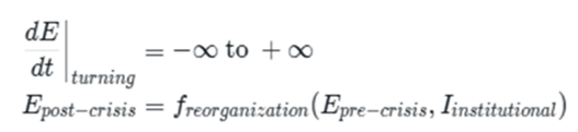
The Turning Point represents the most mathematically fascinating phase, explicitly incorporating mathematical discontinuity to represent systemic crisis and reorganization. The equation for Turning Point acknowledges that technological revolutions involve fundamental discontinuities where existing systems break down and new organizational forms emerge.
The infinite derivative represents the mathematical impossibility of predicting exact crisis trajectories using conventional continuous mathematics. However, the reorganization function depends critically on institutional adaptation capacity—society’s ability to develop new institutions, regulations, social norms, and organizational forms that effectively harness technological potential.
The period from 1793 to 1797 marks a turning point in intense political, economic, and social upheaval. The French Revolution and the Napoleonic Wars created massive disruptions in Europe, while the British economic crises led to the development of new financial and industrial management forms.
Political reorganization was severe. Revolutionary threats led to the expansion of government powers, the introduction of new taxation systems, and changes in central-local government relationships. Economic institutions underwent a dramatic transformation—the Bank of England’s 1797 suspension of gold convertibility marked the inception of the first modern fiat currency system. New corporate organization forms emerged, including joint-stock manufacturing companies.
Labor relations were fundamentally reorganized. The Combination Acts (1799-1800) established new legal frameworks while constraining worker organization. Factory discipline became standardized, and technical education emerged to supply skilled workers for expanding industries.
Social institutions adapted to concentrated urban populations. New municipal government forms, public health systems, and educational institutions emerged. Religious organizations adapted their practices and doctrines to meet the needs of industrial workers, thereby creating new forms of social organization and cultural expression.
The mathematical discontinuity reflects the impossibility of predicting specific institutional innovations from pre-crisis conditions. However, the framework suggests that some form of reorganization was inevitable, given the accumulated tensions between technological capabilities and existing organizational forms.
Reviewing the Turning Point variables
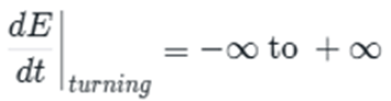
The first equation, dE/dt|_turning = -∞ to +∞, uses mathematical notation to describe something that might seem impossible: an instantaneous change from negative infinity to positive infinity. In mathematical terms, this is called a “discontinuity” or a “singularity”—a point where the standard mathematical rules break down. But what does this mean in human terms?
The “dE/dt” represents the rate of change of energy over time—essentially, how quickly things are changing. During regular periods, this rate of change is finite and predictable. Even during the chaotic Installation Period, despite all the boom-and-bust cycles, the changes follow mathematical patterns. But at the Turning Point, the rate of change becomes infinite in both directions. Old systems collapse instantly while new systems emerge just as quickly. The mathematical discontinuity captures the human experience of a sudden, dramatic transformation that seems to happen overnight.
But why do these discontinuities occur at this point in the technological cycle? The answer lies in understanding how the energy of the Installation Period creates unsustainable tensions that eventually must be resolved. During the railway installation period, the new technology was creating massive social and economic changes. However, the political and institutional structures of society were still based on the old agricultural and craft-based economy.
The mathematical discontinuity occurs when this pressure becomes too great to be contained within existing structures. The old system does not gradually evolve—it breaks. And when it breaks, it breaks suddenly and completely. This is why the rate of change approaches infinity: the transformation happens so quickly that it seems instantaneous.

But discontinuity is not just about destruction—it’s also about creation. The second part of our mathematical framework captures this: E\post-crisis = f\reorganization(E\pre-crisis, I\institutional). This equation describes how the energy that existed before the crisis gets reorganized into new forms after the crisis.
E\post-crisis represents the energy state of society after the Turning Point. This is not necessarily less energy than before the crisis—it is energy that has been reorganized and channeled into new structures.
Epre-crisis is the energy state before the crisis—all the tensions, conflicts, and contradictions that built up during the Installation Period. This energy does not disappear during the crisis; it gets transformed.
I\institutional represents the institutional adaptation capacity of society—its ability to create new institutions that can channel the energy of the technological revolution constructively. This is perhaps the most crucial variable in determining whether a Turning Point leads to positive transformation or destructive chaos.
The function f\reorganization describes how the reorganization process works. This is not a simple mathematical relationship but rather a complex process involving political negotiation, social conflict, institutional innovation, and cultural adaptation. The specific form this function takes depends on the historical circumstances. Still, the general pattern is consistent: old institutions that cannot handle the energy of the new technology are replaced by new ones that can.
The mathematics of the Turning Point also explains why these periods are so brief compared to the other phases. The discontinuous nature of the transformation means that it happens quickly, usually within a few years. Society can’t sustain the infinite rate of change for long. Either the transformation succeeds, and new stable institutions emerge, or it fails, and society collapses into chaos.
Understanding the mathematics of the Turning Point helps us recognize that the crises that mark these periods aren’t signs of failure but necessary stages in the process of technological transformation. The discontinuity is required to break down old structures that are incompatible with the new technology and create space for new institutions that can harness its potential.
The mathematics of discontinuity reminds us that technological revolutions are not just about technology—they are about the complete reorganization of society. The Turning Point is where this reorganization happens, and its mathematical nature as a discontinuity explains why these periods are so dramatic, so consequential, and so brief.
Deployment Period
Golden Age and Gradual Exhaustion
The Deployment Period represents the mature technological cycle phase, characterized by sophisticated dynamics capturing the complex interplay between golden age productivity growth and gradual technological exhaustion. The equation for Deployment incorporates competing processes: sustained productivity improvements through systematic optimization, learning curve effects from accumulated experience, and gradually increasing constraints as core technology applications are exhausted.
The mathematical structure begins with maximum energy potential established during the Turning Point reorganization. The golden age component describes sustained productivity growth through mature deployment within optimized institutional frameworks. The learning curve component reflects gradual optimization through experience and incremental improvement, while the exhaustion decay term represents gradual depletion of growth opportunities within the existing paradigm.
Following the institutional reorganization of the 1790s, Britain entered a period of sustained industrial growth, marking the mature realization of technological possibilities. Manchester cotton production increased from 50 million pounds (1798) to 350 million pounds (1820)—8.7% annual growth achieved through systematic optimization rather than breakthrough innovations.
Production costs fell dramatically through systematic optimization. Cotton yarn prices decreased from 7 shillings per pound (1798) to 2 shillings (1820)—a 65% reduction through learning curve effects and operational improvements, while quality simultaneously improved.
Steam power proliferated from approximately 1,200 units (1798) to over 15,000 (1829), with growth patterns showing gradual saturation characteristic of mature technology deployment. Power output per engine increased from 15 horsepower (1798) to 40+ horsepower (1829) through incremental engineering improvements and operational optimization.
Infrastructure development demonstrated a systematically established technology application. Canal mileage increased from 1,200 to 4,000 miles, creating national transportation networks, reducing shipping costs, and enabling economic specialization. Road improvements reduced travel times by 40-60% over major routes.
However, signs of technological exhaustion became apparent by the 1820s. Capital productivity in textiles peaked around 1815-1820, then declined as new construction required increasingly sophisticated technology for competitive returns. Market saturation effects emerged as domestic basic textile demand was largely satisfied. Innovation rates in core technologies peaked in the 1810s and then declined steadily through the 1820s.
The mathematical framework successfully captures this dual nature through the combination of growth and decay terms. Total factor productivity in manufacturing grew at 2.5% annually (1798-1829) compared to 0.8% pre-industrial, tripling the improvement rate. Labor productivity improvements were dramatic: textile workers in 1829 produced approximately 15 times more than in 1798, representing 9.2% compound annual growth.
Reviewing the Deployment period variables
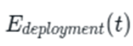
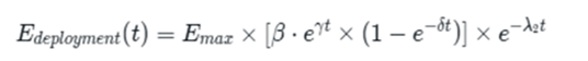
E\deployment(t) represents the total productive energy of society during the Deployment Period. This is different from the chaotic energy of the Installation Period. During Deployment, energy flows in organized, productive channels. It builds infrastructure, creates wealth, expands trade, and generally improves human welfare. During the steam and railway Deployment Period, this energy manifested as the rapid expansion of railway networks, the growth of industrial cities, the development of international trade, and the general prosperity that characterized by the era.

E\max represents the maximum potential energy that the technology can deliver. This is the theoretical upper limit of what the textiles and canals revolution could achieve. The basic principles were established, the major technical problems were solved, and the institutional framework was in place.

The most mathematically interesting part of the equation is the middle section: \[β · e^(γt) × (1-e^(-δt))]. This complex expression describes the characteristic dual-phase nature of Deployment Periods: a Golden Age of rapid improvement followed by a period of maturation and approaching limits.
Let’s start with β (beta), which represents the “golden age amplification factor.” This captures the efficiency gains that result from society finally learning how to utilize the new technology effectively. During the Installation Period, much of the energy was wasted on speculation, redundant construction, and inefficient experimentation. But during the Deployment Period, society has learned from its mistakes. Best practices have been established, efficient institutions have been created, and the technology is being used to its full potential. The beta factor amplifies the underlying technological potential.
The term e^(γt) represents exponential growth driven by continuous improvement and optimization. The γ (gamma) is the productivity growth rate—the speed at which society gets better at using the technology.
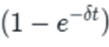
But the exponential growth term is multiplied by (1-e^(-δt)), which represents a learning curve that approaches a limit. The δ (delta) is the learning curve parameter. This mathematical expression starts at zero and gradually approaches one, creating an S-shaped curve. In practical terms, this captures the fact that improvements come quickly at first but become harder to achieve over time. The easy gains are made first, and each subsequent improvement requires more effort and investment.
During the deployment period, we can see this learning curve. In the early years, dramatic improvements were common. However, by the 1820s, the rate of improvement had slowed. Further improvements were still possible, but they were incremental rather than revolutionary.

The final term, e^(-λ₂t), represents the gradual exhaustion of the technology’s potential. This is an exponential decay function, similar to what we saw in the Installation Period, but with a different decay constant λ₂ (lambda-2). While the technology continues to improve and expand, it’s gradually approaching its limits. The low-hanging fruit has been picked, and the remaining opportunities are increasingly difficult and expensive to exploit.
This mathematical structure creates a characteristic pattern: rapid growth that gradually slows as the technology matures and approaches its limits. The combination of exponential growth and exponential decay creates what mathematicians call a “logistic curve”—fast growth that levels off as it approaches a maximum.
The mathematical beauty of the Deployment equation is that it explains why Golden Ages are both extraordinary and temporary. The same mathematical forces that create the golden age also ensure that it cannot last forever. Exponential growth creates prosperity, but the learning curve ensures that the rate of improvement will eventually slow. The exhaustion term ensures that the technology will eventually reach its limits.
By 1829, the textiles and canals revolution was mathematically exhausted. The easy improvements had been made. The institutional framework was mature. The technology was still helpful and productive, but it was no longer revolutionary. The energy that had driven the transformation was dissipating, and society was ready for the next technological revolution.
But the equation reveals another crucial insight: the Deployment Period doesn’t end with collapse but with a gradual transition. The exponential decay is slow and gentle, unlike the chaotic energy burns of the Installation Period. This gives society time to adapt and prepare for the next wave of innovation. The prosperity created during the Golden Age provides the resources and stability needed for the next phase of Core Formation to begin.
This mathematical understanding of the Deployment Period helps us recognize that technological revolutions are not just about single technologies but about waves of innovation that were essentially industry cores built upon each other. The gradual exhaustion of one revolution creates the conditions for the next, and the mathematics ensures that this process continues indefinitely.
The Deployment equation also helps us understand the social and political characteristics of the Golden Ages. The mathematical stability of the period—the fact that exponential growth is balanced by learning curves and gradual exhaustion—creates social stability. Unlike the chaos of Installation Periods or the discontinuity of Turning Points, Deployment Periods are characterized by steady, predictable improvement. This makes the social conditions for cultural flowering, institutional development, and general prosperity that we associate with the Golden Ages.
To get you to the equations as quickly as possible, this chapter has been laid out backwards. A quick introduction to the structure of the technology cycles is provided at the top of the equations and their explanations. What follows is the synthesis of the evolution, all the periods dated, finishing with where the ideas came from for the equations.
The Hidden Architecture
In 1687, Isaac Newton revealed that an apple falling from a tree follows the same mathematical laws that govern the orbits of planets. Three centuries later, we stand on the verge of an equally revolutionary insight: human technological progress operates according to mathematical principles as fundamental and elegant as the laws of physics themselves.
This is not a metaphor. It is a precise mathematical framework that explains why civilizations experience technological revolutions in distinct cycles, why innovations cluster together before exploding into transformative periods, and why each revolution follows predictable phases of chaos, crisis, and golden age productivity. Most remarkably, it reveals that technological evolution operates according to conservation laws that may be as fundamental to the universe as the conservation of energy and mass.
What you are about to discover challenges our most basic assumptions about human progress, suggesting that consciousness itself might be the universe’s method for converting matter and energy into ever-greater complexity through precisely orchestrated technological cycles.
The Evolution of Technology
Imagine if technological progress followed the same fundamental laws as the universe itself—where innovations cluster together like matter before the Big Bang, explode into transformative cycles like cosmic inflation, and eventually burn out like dying stars, only to seed the next generation of breakthroughs. This is not science fiction. It is the revolutionary framework of the Perez Cycle, which reveals that human technological development operates according to mathematical principles as elegant and predictable as Einstein’s famous equation E = mc².
To understand why this matters, consider the profound mystery that has puzzled historians, economists, and philosophers for generations: Why does human progress unfold in distinct waves rather than smooth, continuous advancement? Why do specific periods in history—the Industrial Revolution, the Railway Age, the Electrical Era—seem to concentrate extraordinary innovation while other periods feel stagnant by comparison?
The answer emerges when we stop thinking of technology as mere tools and start understanding it as a form of energy that follows conservation laws as fundamental as those governing matter and energy in physics. Just as Einstein revealed that matter and energy are interchangeable according to precise mathematical relationships, the Perez framework shows that human consciousness converts accumulated innovations into technological energy through equally precise mathematical processes.
The Mystery of Recurring Revolutions
For centuries, historians and economists have puzzled over a strange pattern in human progress. Approximately every 40-70 years, with remarkable consistency, our civilization experiences a complete technological transformation. The Industrial Revolution (1768-1829) gave way to the Steam & Railway Age (1829-1873), which in turn yielded to the Steel & Electrical Age (1875-1918), followed by the Automobile Age (1908-1974), and most recently, the Information Age (1971-present). Each revolution does not just bring new gadgets—it completely reorganizes how we live, work, and think.
But the pattern runs deeper than mere sequence. Each cycle follows an almost identical mathematical structure: a 30–40-year period of invisible accumulation, a sudden explosive transformation, a chaotic installation period marked by financial bubbles and social disruption, a sharp crisis and institutional adaptation, followed by a golden age of productive deployment that gradually exhausts itself while simultaneously seeding the next revolution.
This regularity suggests something profound: technological evolution isn’t random or even primarily driven by human intention. Instead, it appears to follow mathematical laws as precise as those governing planetary orbits or quantum mechanical states.
The Thermodynamics of Innovation
To understand technological cycles mathematically, we must first grasp how innovation energy accumulates, converts, and dissipates. Like all energy systems in the universe, technological development follows the laws of thermodynamics:
First Law (Conservation of Innovation Energy): The total amount of innovation energy in the universe is constant. It can neither be created nor destroyed, only transformed from potential form (accumulated innovations) to kinetic form (active technological cycles).
Second Law (Entropy of Technological Systems): In any closed technological system, entropy tends to increase over time. Mature technologies become increasingly complex, inefficient, and fragmented, creating the disorder that drives the formation of the next innovation cluster.
Third Law (Absolute Zero of Innovation): As any technological system approaches its fundamental limits, the rate of innovation approaches zero. This creates a mathematical boundary condition that forces the formation of entirely new technological paradigms.
These laws explain why technological progress cannot be smooth and continuous. Just as water cannot gradually transition from ice to steam without the distinct phase change of boiling, human civilizations cannot gradually transition between technological paradigms without the different phase changes we call technological revolutions.
The Physics of Innovation
Where Ideas Become Energy
At the heart of this new understanding is a deceptively simple equation that mirrors Einstein’s most famous discovery:
E = Mc²
However, instead of matter converting to energy, this describes how industry-clustered innovations evolve into the monster technological cycles. Here, E represents the total energy available to power an entire technological revolution. M represents the “mass” of innovations that have clustered together during a preparatory period. And c² represents the speed at which technological transformation can spread through human civilization.
Think of it this way: just as Einstein showed that a small amount of matter can release enormous energy when conditions are right, the Perez framework reveals that a relatively small cluster of breakthrough innovations can release enough transformative energy to power decades of civilizational change, worldwide, no less.